A Stat Arb on Crypto Tokens
A mean-reversion strategy on 40 crypto tokens, built from the Avellaneda–Lee (2010) playbook. My first version posted a positive Sharpe ratio and still turned $1 into $0.00000005. This page walks through the idea, the build, what broke, and what the corrected version really shows.
The idea
Crypto tokens move together. When Bitcoin rallies, most of the market rallies with it. That shared movement is the tide, and it lifts every boat at once. Once you strip the tide out, what remains for each token is its own story: the part of its return that has nothing to do with the market.
Statistical arbitrage bets that this leftover part behaves like a rubber band. It gets stretched by noise, flows and news, and then it tends to snap back. When a token is unusually cheap relative to what the market says it should be, you buy it. When it is unusually rich, you short it. You close the trade once the band relaxes.
Marco Avellaneda and Jeong-Hyun Lee formalised this for US equities in 2010. I applied their method to crypto, trading hourly across a one-year window from 26 September 2021 to 25 September 2022.
The data
Two files drive everything. The first holds hourly prices for more than 120 tokens. The second lists, for every hour, the 40 largest tokens by market capitalisation at that moment. The universe therefore changes over time: tokens enter the top 40 and fall out of it.
For every hour \(t\) I look back over a window of \(M = 240\) hours (ten days). I keep only the current top-40 tokens that have at least 80% valid data in that window. Returns are simple hourly returns:
\[R_{i,t} = \frac{S_{i,t} - S_{i,t-1}}{S_{i,t-1}}\]The method, in four steps
The same four steps repeat every hour, 8,760 times.
Step 1: Find the tides with PCA
I standardise each token's returns inside the window and compute their correlation matrix. Principal component analysis then finds the directions in which the whole market moves together. I keep the top two eigenvectors \(v^{(1)}\) and \(v^{(2)}\).
To turn an eigenvector into something tradable, each token's loading is divided by its volatility \(\bar{\sigma}_i\). The result is an eigenportfolio, and its return is the factor return:
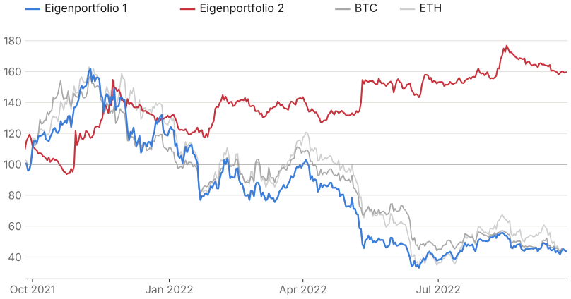
\[Q^{(j)}_i = \frac{v^{(j)}_i}{\bar{\sigma}_i}, \qquad F_{j,k} = \sum_{i=1}^{N} Q^{(j)}_i \, R_{i,k}\]The first eigenportfolio behaves like the market. Every token carries a positive weight, and over the year it tracks Bitcoin almost exactly.
Source: FTX hourly prices
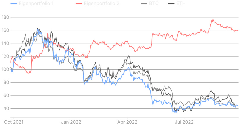
The first eigenportfolio fell 56% over the year, in line with Bitcoin and Ether. The second went the other way and rose 60%. It is a relative-value factor: long some tokens, short others.
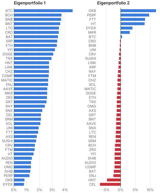
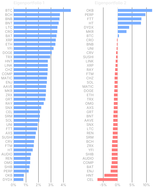
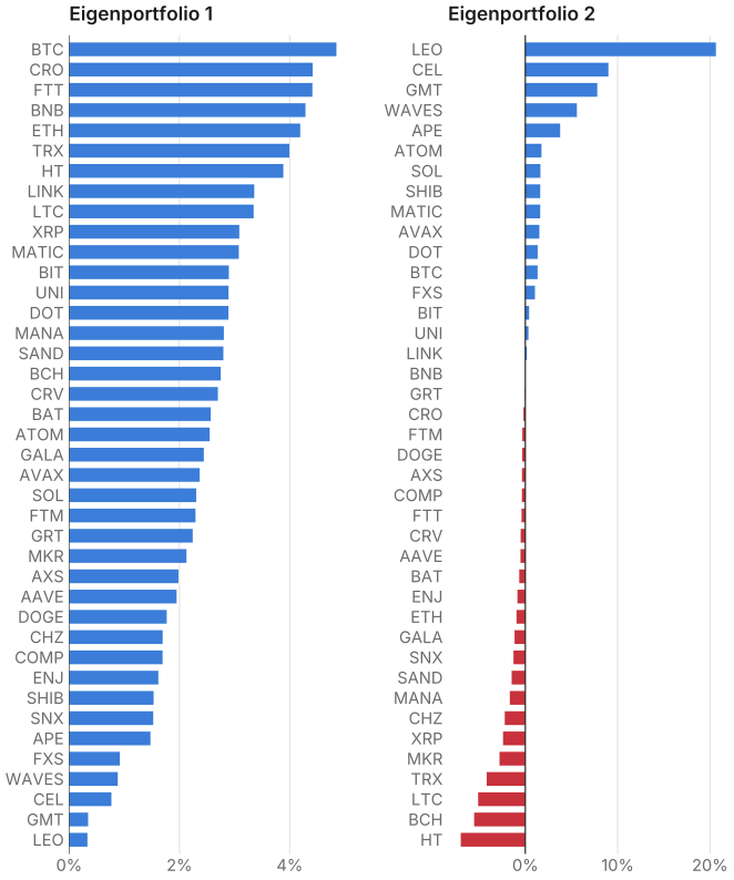
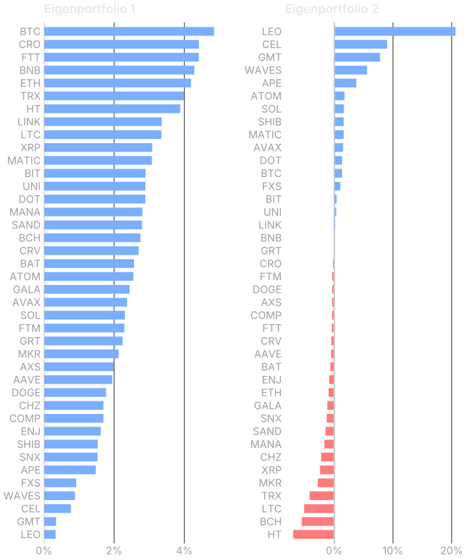
The weights show the same thing from another angle. The first eigenportfolio spreads positive weight across the whole universe, with Bitcoin the largest. The second concentrates on a handful of tokens, some held long and some short.
Source: FTX hourly prices
Source: FTX hourly prices
The second factor tends to lean heavily on a few thinly traded, exchange-linked tokens such as LEO and CEL. That makes it less stable from hour to hour than the market factor, and it is a hint that a liquidity screen would help.
Step 2: Strip out the tides
For each token I regress its returns in the window on the two factor returns:
\[R_{i,k} = \beta_{i,0} + \beta_{i,1} F_{1,k} + \beta_{i,2} F_{2,k} + \varepsilon_{i,k}\]The betas measure how much the token rides each tide. The residual \(\varepsilon_{i,k}\) is its idiosyncratic return, the part that is purely about that token.
Step 3: Model the residual as a rubber band
Adding up the residuals gives a running total, which measures how far the band is stretched:
\[X_{i,\ell} = \sum_{n=0}^{\ell} \varepsilon_{i,\,t-M+n}\]The mathematical rubber band is the Ornstein–Uhlenbeck process. It is pulled back towards an equilibrium level \(m\) at speed \(\kappa\) while random shocks keep jostling it. I estimate it through an AR(1) regression, which is simply its discrete-time version:
\[X_{\ell+1} = a + b\,X_\ell + \zeta_{\ell+1}\]The AR(1) coefficients translate directly into the OU parameters, with \(\Delta t\) equal to one hour expressed in years:
\[\kappa = -\frac{\ln b}{\Delta t}, \qquad m = \frac{a}{1-b}, \qquad \sigma_{\text{eq}} = \sqrt{\frac{\operatorname{Var}(\zeta)}{1-b^2}}\]A coefficient \(b\) close to 1 means a weak pull, where the band barely snaps back. Fits with \(b \ge 0.999\) show no usable mean reversion, so I discard them.
Step 4: Score the stretch and trade it
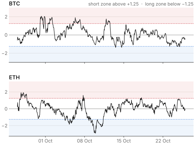
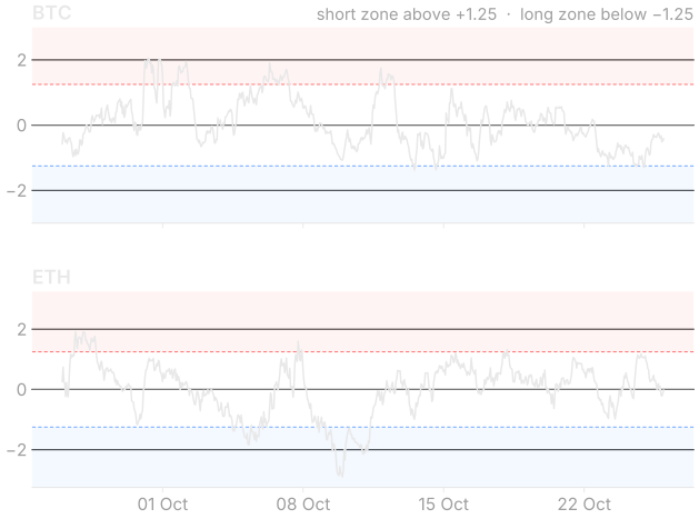
The s-score measures how many equilibrium standard deviations the band currently sits from its resting point:
\[s_i = \frac{X_{i,\text{last}} - m_i}{\sigma_{\text{eq},i}}\]I subtract the cross-sectional average each hour so the scores are centred on zero. The trading rules follow the paper. Buy when \(s < -1.25\) (too cheap) and close the long once \(s > -0.50\). Short when \(s > +1.25\) (too rich) and close once \(s < +0.75\). Every signal acts on the following hour's return, so the backtest never peeks at the future.
Source: FTX hourly prices
How the code is organised
The whole pipeline lives in a single Python script built around three classes. DataHandler loads prices, computes returns, and builds each hour's filtered window. FactorModel runs the PCA and produces eigenportfolio weights and factor returns. OUProcess runs the factor regression, fits the AR(1), maps it to OU parameters, and returns an s-score. A backtest driver loops over the 8,760 hours, applies the trading rules, and writes the signals, weights, performance statistics and charts. Keeping these pieces separate made it easy to find and fix problems later, which turned out to matter.
The first result: a positive Sharpe ratio, and total ruin
My submitted version reported a Sharpe ratio of 0.13 and a maximum drawdown of −100%. On average the strategy made money every hour. Compounded, it lost essentially everything: $1 invested at the start was worth $0.00000005 at the end.
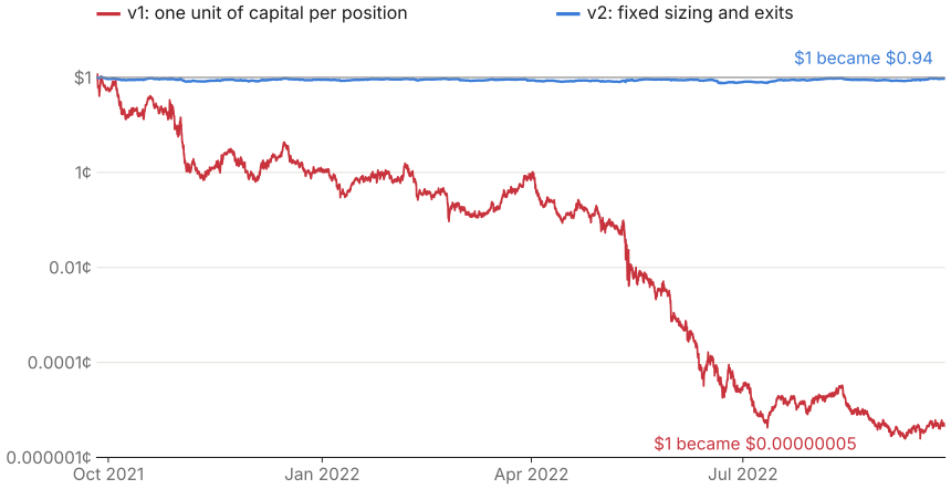
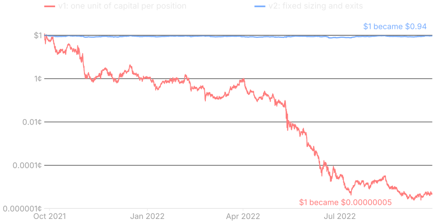
Source: FTX hourly prices
At the time I put this down to missing transaction costs. When I revisited the project, the real explanation turned out to be three implementation mistakes.
What went wrong
Every position was sized as if it were the whole portfolio
Each open position was worth one unit of capital, and on average 23 positions were open at once. That is roughly 23 times leverage on a portfolio worth 1. The portfolio moved more than 10% in about one hour out of every twelve.
This explains how a positive average return can coexist with ruin. A compounded portfolio grows at roughly its mean return minus half its variance:
\[\text{growth rate per hour} \approx \mu - \tfrac{1}{2}\sigma^2\]Version one averaged \(\mu \approx 0.009\%\) per hour, with \(\sigma \approx 6.3\%\) per hour. The volatility drag \(\tfrac{1}{2}\sigma^2 \approx 0.20\%\) per hour was more than twenty times the drift. The Sharpe ratio measures the average and cannot see the drag, but the drag is what compounding feels.
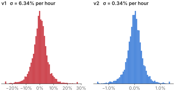
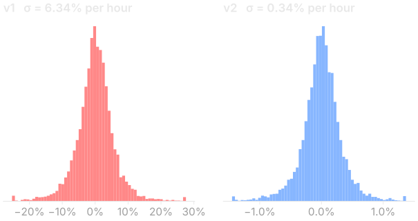
Source: FTX hourly prices
Positions were orphaned when tokens left the universe
The trading loop only updated tokens that were in that hour's top-40 window. When a token dropped out, its position froze. It kept earning and losing money, but the model never looked at it again and never closed it. More than a third of all position-hours (36%) sat in tokens the model had stopped tracking. One token, C98, was held for 8,588 of the 8,760 hours.
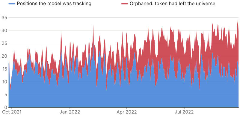
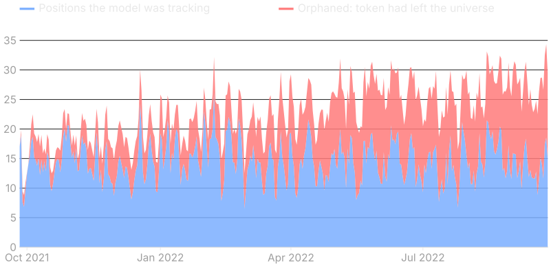
Source: FTX hourly prices
The eigenportfolios were never normalised
Dividing each loading by an hourly volatility of 1–5% inflates the weights, which summed to around 600. The first factor's return was therefore about 600 times the average token's move. This did not affect the regressions, because rescaling a regressor leaves its residuals unchanged. It did make the original factor chart unreadable. Scaling each eigenportfolio to unit gross weight fixed it.
After the fixes: honest, and flat
I changed three things. Positions are now equally weighted so gross exposure is always 1. Any position in a token that leaves the universe is closed. Factor returns are reported on unit-weight eigenportfolios.
| Version one | Version two | |
|---|---|---|
| Total return | −100% | −5.6% |
| Annualised Sharpe ratio | 0.13 | −0.02 |
| Maximum drawdown | −100% | −26% |
| Annualised volatility | 593% | 32% |
| Average open positions | 23 | 15 |
The corrected strategy survives, but it has no edge: the mean hourly return is essentially zero. Costs make things worse. The strategy turns over its book roughly 1,100 times a year, so a cost of just 5 basis points per trade would have cut the return to −46%.
What I take away
The most useful lesson was the gap between the arithmetic average and compounded wealth. A Sharpe ratio built from average returns can look respectable while the portfolio underneath is being destroyed by its own volatility. Position sizing is not a detail to add after the signal works. It decides whether the signal can be felt at all.
The second lesson is about bookkeeping. A dynamic universe needs an explicit rule for what happens to a position when its asset leaves, and it is exactly the kind of bug that is invisible until you count.
On the signal itself, mean reversion in hourly crypto residuals did not pay over this year, which was a brutal bear market that included the Terra collapse. If I took this further, I would try four things. First, require faster mean reversion, since the paper insists the reversion time be short relative to the estimation window. Second, add a liquidity screen. Third, scale signals by trading volume, as Avellaneda and Lee do. Fourth, trade less often so that turnover does not eat whatever edge exists.
References
- Avellaneda, M., & Lee, J.-H. (2010). Statistical arbitrage in the US equities market. Quantitative Finance, 10(7), 761–778.